Econometric Advisors' blog

By Christina Tong, Stefan Weiss, Tyler Mangin, Ph.D.

Executive Summary

CBRE Econometric Advisors (CBRE EA) now offers a stand-alone effective rent series for the office sector, covering 61 U.S. markets including 834 submarkets on a quarterly basis with data going back to Q4 2010.

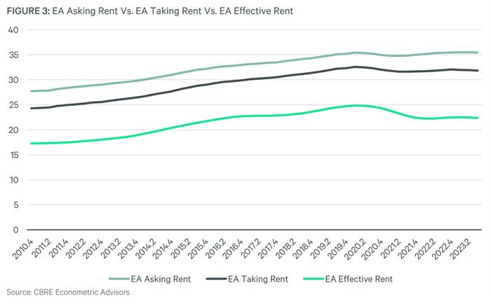
The EA Effective Rent series is based on a net present value (NPV) analysis incorporating base rent, term, escalations, free rent, tenant improvement allowances, and a discount rate equal to the long-run returns of the NCREIF office index. We then apply a payment function to identify the fixed rent that has the same NPV as the actual stream of cashflows.

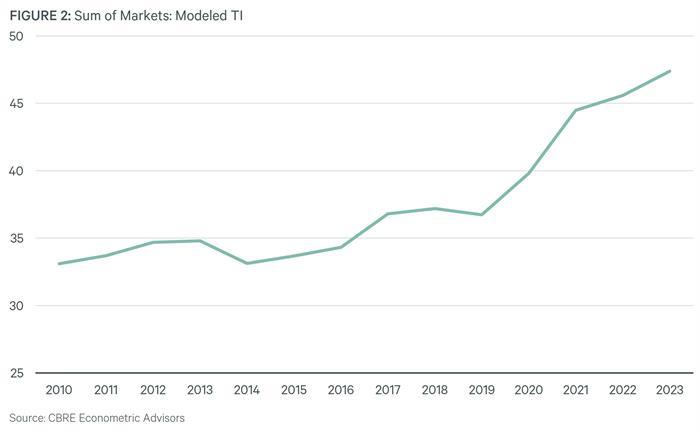
Tenant Improvement Allowances (TIs) are the most frequently discussed and most nebulous of the deal terms that impact effective rent calculations. Unsurprisingly, they were the most complicated to model. Along with individual deal and market factors, we were excited to find that both lagged real Treasury bond yields and lead inflation expectations were significant in predicting deal level TIs.

A recap of the EA Taking Rent Methodology

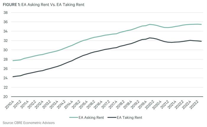
Leveraging CBRE proprietary voucher data, CBRE EA uses a panel model to predict the gap between asking rent and taking rent. EA’s ability to match individual transactions to suite-level asking rent at the time of transaction allowed for the mapping out of an ask-to-take discount percentage for nearly every transaction in our database. We then modeled how key factors influence and drive this discount, landing at a model for the ask-to-take discount that utilizes deal level factors (lease size, lease term, and lease’s matched asking rent) as well as market level factors such as the vacancy rate and asking rent. This modeled discount is then applied to the EA Asking Rent series to form the EA Taking Rent series (Figure 1).

What is EA Effective Rent?

The EA Taking Rent series was a pivotal step toward an EA Effective Rent series. In addition to accounting for lease term, rent escalations, free rent concessions, and tenant improvement allowances, a key component of an effective rent series is the ability to account for the time value of money. To do this we construct a discount rate which reflects the opportunity cost of capital for the office investment. A return that an investor would expect to gain in other investments of similar risk. Aggregating each of these components via the equation below allows us to compare different transactions with different cash flow schedules to accurately assess the relative value of each transaction (and most importantly, how that ‘true value’ is changing over time and across markets):

Effective Rent = (i )/〖1-(1+i)〗^(-n) ∗ (-TI+R_t/(1+i)^t +R_((t+1) )/(1+i)^(t+1) +R_((t+2) )/(1+i)^(t+2) +…+R_((n))/(1+i)^n )

Where i = Discount rate

           R_t = net cash flow per sf at time t

           T = 1,t time period

  TI= Tenant Improvement

  N= number of years (standardized to a 7-year term)

Modeling the components of EA Effective Rent

e. Tenant Improvement Allowance (TIs) – TIs are the most frequently discussed and most nebulous of the deal terms that impact effective rent calculations. For simplicity, TIs are recognized at the onset of the lease (at time period T=0).

The TI Model

To model TIs, we leveraged a generalized linear model (GLM) with a Poisson distribution and a log link function. This best fitting model is represented by the equation:

〖log⁡(E(TI〗_jt)) =β0+ β1∗〖LeasingSF〗_jt+ β2∗〖Term〗_jt+β3∗〖TakingRent〗_jt+β4∗〖RealRentGrowth〗_t+β5∗〖RealLagTbond〗_t+β6∗〖LeadInflation〗_t+MarketFE  

Where;

  〖TI〗_jt = Tenant Improvement Per s.f. for deal j at time t

  〖LeasingSF〗_jt = lease square feet for deal j at time t

  〖Term〗_jt = lease term in years for deal j at time t

  〖TakingRent〗_jt = Taking rent for deal j at time t

  〖RealRentGrowth〗_t = inflation adjusted asking rent growth at time t

  〖RealLagTbond〗_t  = 10-Year Real Treasury Bond Rate at time t-1

  〖LeadInflation〗_t  = Lead 1-Year Inflation rate at time t

  MarketFE= Market level fixed effect

   t =1,T time periods

  j= 1,N deals

Aside from being statistically significant, the inclusion of the lagged real Treasury bond makes sense as the cost of capital influences an owner’s decisions to ‘lend’ by way of an expensive buildout package. There is also, generally, a substantial lag between when a lease is negotiated and when the final lease is signed.

A similar logic applies to the inclusion of inflation on a one-year lead, as a tenant’s actual cost to construct a buildout assumes expectations of inflation throughout the construction period.

As a last step, we take the coefficients outputted from this model and feed in the market-level taking rent, a fixed lease size to 20,000 sq. ft. and a lease term of seven years. Once again, fixing size and term allows us to standardize and compare the TI (and by extension effective rents) across markets.

Putting it all together: EA Effective Rent

Estimating equation 2 gives us the TI values needed to construct an effective rent series going back to 2010 across all 61 of EA’s Tier 1 markets. While every deal contains its own nuances, for simplicity TIs are recognized in period 0 and free rent is recognized in period 1. We then calculate the NPV of the stream of cashflows using an 8.2% discount rate. Lastly, use a simple payment function to identify the fixed payment which, at the same 8.2% discount rate, has the same present value as the actual stream of cash flows.

To ensure a more robust sample, the EA Effective Rent was first modeled on an annual basis and then a quarterly series was interpolated using a cubic spline function.

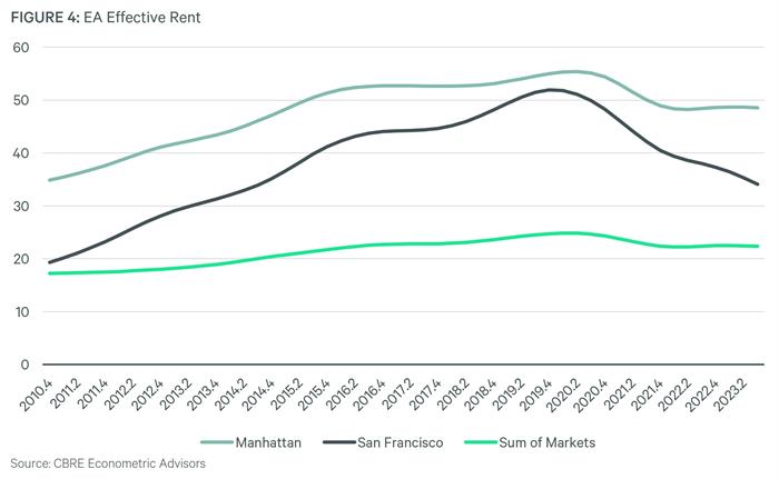
To gain more granularity, we share down the market level EA Effective Rent to submarkets using the market level relationship between vacancy and effective rent/taking rent discount as a guide. To reduce the impact of vacancy volatilities, we put guardrails on the movement of the effective rent discount based on the submarket’s correlation with the broader market. Submarkets with more volatile vacancy movements will have discounts that more closely match the broader market, and vice versa.

What does the EA Effective Rent series tell us?

a. Changes over time: While asking rents across EA’s Sum of Markets have returned to their Q1 2020 level, EA Effective Rents have fallen 10.0% during that time. Further, the national EA Effective Rent figure now represents a 37% discount to EA Asking Rents, and a 30% discount to EA Taking Rents. This compares to 2019 when the ask-to-effective discount was tighter at 30%.

b. Spread of different markets: The variation among markets is also more truly defined in EA Effective Rents. This is important because different markets are showing different mechanisms for absorbing market weakness. The value in an Effective Rent series is the ability to normalize and compare each of those mechanisms in a single, holistic equation. For example, in Atlanta asking rents have increased 4%, but the combination of concessions and post-negotiation discounts have caused effective rents to fall 11%. Conversely, in Manhattan asking rents have fallen 5.4% - notably more than the national figure, which has been flat. But the decline in effective rents is comparable at 12.2% for Manhattan compared to 10.0% nationally. We also see in markets like San Francisco, which was hit extraordinarily hard by hybrid work’s impact on the tech sector, not only are asking rents down 17% since the start of the pandemic but effective rents are down 34%. EA Effective Rents are picking up the nuances across markets, normalizing various methods for capturing fundamentals, and allowing for the first time an apples-to-apples comparison of true rental income across both space and time.

The Future

While the EA team is proud to be releasing the EA Effective Rent series to office sector subscribers, we are rapidly pushing the next round of exciting updates. These include:

a. Prime Effective Rents: leveraging EA’s newly released prime office series, the above methodology can be used to predict taking rent and effective rent in prime office buildings.

b. EA Effective Rents in other sectors.

c. EA Net Effective Rent - leveraging data on operating expenses, we’re able to release a fourth series net of OpEx and taxes. This answers that final question related to ‘the bottom line’. With the EA Net Effective Release, EA clients will have, by market and submarket, data on asking rents, taking rents, effective rents, and net effective rents.